Lesson 03 - NumPy and pandas
Lesson 03 - NumPy and pandas
So far we have covered the base Python environment - built in data types and structures, and looked at how we can use Python as a general purpose programming language.
Now we will hone in on our goal of data science - using the data science modules developed by the data science community. Download todays notebook here.
This lesson and the next lesson are based on the book Python for data analysis, by Wes McKinney, the primary developer of pandas. Feel free to go without the book - we will cover much of its content in the class, and it is a little outdated.
The first module we will examine is NumPy and we will the move onto pandas. NumPy provides arrays, while pandas provides DataFrames.
NumPy
NumPy stands for numerical Python. So far the Python data structures have worked, but have not been tailored for large scale data analysis.
Think of how Python works under the hood when multiplying every element of a list by 2:
In [1]:
l = [1,2,3,4,5]
print(l*2)
#probably not what we want as statisticians!
print([i *2 for i in l])
#this works, but what about -
l = [1,2,3,4,'a']
print([i *2 for i in l])
[1, 2, 3, 4, 5, 1, 2, 3, 4, 5]
[2, 4, 6, 8, 10]
[2, 4, 6, 8, 'aa']
Python needs to check each data type to find the times method associated with it. In small examples like this, the overhead is very low, but when we are dealing with millions of rows, it quickly adds up.
To work better with numeric (or other large scale data), numpy introduces the array, a data structure which may only contain one type of data:
In [9]:
import numpy as np
l = [1,2,3,4,5]
k = np.array(l)
print(k * 2)
[ 2 4 6 8 10]
It is also much faster (by a process called vectorisation):
In [3]:
l = range(10000)
k = np.array(l)
%timeit [i * 2 for i in l]
%timeit k * 2
100 loops, best of 3: 2.1 ms per loop
10000 loops, best of 3: 57.6 µs per loop
As well as the array data type, numpy contains broadcasting methods, built in functions utilising the array structure to work extremely fast (by going through C), linear algebra, random numbers and good integration into C and Fortran code
NumPy basics
The array is a new class, with a lot of its own methods. The exact implementation is outside the scope of the class, take a look at the NumPy website for source code and official documentation.
Technically, we use the np.array to create an instance of class ndarray. I’ll refer to them as arrays in this lesson.
We can access the type of data contained in an array:
In [4]:
a = np.array([1,2,3,4,5])
print(a.dtype)
print(np.sctypes)
int64
{'float': [<class 'numpy.float16'>, <class 'numpy.float32'>, <class 'numpy.float64'>, <class 'numpy.float128'>], 'others': [<class 'bool'>, <class 'object'>, <class 'str'>, <class 'str'>, <class 'numpy.void'>], 'complex': [<class 'numpy.complex64'>, <class 'numpy.complex128'>, <class 'numpy.complex256'>], 'int': [<class 'numpy.int8'>, <class 'numpy.int16'>, <class 'numpy.int32'>, <class 'numpy.int64'>], 'uint': [<class 'numpy.uint8'>, <class 'numpy.uint16'>, <class 'numpy.uint32'>, <class 'numpy.uint64'>]}
We can initialise arrays in a number of ways
In [8]:
#empty - uninitialised, random numbers!
print(np.empty((2, 3, 2)))
#all zeros
print(np.zeros((3, 6)))
#from a list
print(np.array([1,2,3,5]))
#arange is the numpy version of range - gives an array
print(np.arange(10))
[[[ 6.90469329e-310 2.13249800e-316]
[ 0.00000000e+000 0.00000000e+000]
[ 0.00000000e+000 8.60952352e-072]]
[[ 4.46535817e-090 1.39938874e-076]
[ 1.55075695e+184 1.43927482e+160]
[ 3.99910963e+252 2.32204073e-056]]]
[[ 0. 0. 0. 0. 0. 0.]
[ 0. 0. 0. 0. 0. 0.]
[ 0. 0. 0. 0. 0. 0.]]
[1 2 3 5]
[0 1 2 3 4 5 6 7 8 9]
In [205]:
#can specify data type
arr1 = np.array([1, 2, 3], dtype=np.float64)
#and cast it:
arr1.astype(np.int32)
#changing type copies, rather than modifies in place
array([1, 2, 3])
In [25]:
#numpy is vectorized!
print([1,2,3,4] *2)
print(np.array([1,2,3,4]) *2)
#we do this by broadcasting....
[1, 2, 3, 4, 1, 2, 3, 4]
[2 4 6 8]
In [10]:
print(np.array([1,2,3,4]) * np.array([1,2,3,4]))
#times, / etc
#this is not matrix multiplication!!
print(np.array([[1,2],[3,5]]) * np.array([[1,2],[3,5]]))
[ 1 4 9 16]
[[ 1 4]
[ 9 25]]
Subsetting
We can subset much like lists, with the addition of broadcasting for assignment
In [217]:
l = list(range(10))
l[2:5] = 3
print(l)
#error!
l = np.arange(10)
l[2:5] = 3 #broadcasting
print(l)
---------------------------------------------------------------------------
TypeError Traceback (most recent call last)
<ipython-input-217-3d54943f2f76> in <module>()
1 l = list(range(10))
----> 2 l[2:5] = 3
3 print(l)
4 #error!
5 l = np.arange(10)
TypeError: can only assign an iterable
We need to be careful about assigning slices:
In [218]:
#linked! reference
l = np.arange(10)
l_slice = l[5:8]
l_slice[:] = 4
print(l)
#use .copy()
[0 1 2 3 4 4 4 4 8 9]
We can make 2d and 3,4,5… matrices using nested lists, and subset them appropriately:
In [13]:
#nested lists are made to be 2d
arr2d = np.array([[1, 2, 3], [4, 5, 6], [7, 8, 9]])
print(arr2d.shape)
print(arr2d.ndim)
arr2d[1][1]
arr2d[1,1]

arr2d[1:,2:]
arr2d[1,2:]
#multid
arr = np.array([[[1, 2, 3], [4, 5, 6], [7, 8, 9]],[[1, 2, 3], [4, 5, 6], [7, 8, 9]]])
print(arr.shape)
print(arr.ndim)
#broadcasting - must match or be one in each dimension!
arr * np.array([[[1,2,3],[4,5,6],[7,8,9]]])
(3, 3)
2
(2, 3, 3)
3
array([[[ 1, 4, 9],
[16, 25, 36],
[49, 64, 81]],
[[ 1, 4, 9],
[16, 25, 36],
[49, 64, 81]]])
In [30]:
#on multi dimensional arrays, we can use axis calls to do things by rows or columns:
arr2d.sum()
arr2d.sum(axis = 0)
arr2d.sum(axis = 1)
array([ 6, 15, 24])
We don’t need filter: We can subset with booleans much like R:
In [17]:
#no filter, just use booleans
l = np.random.randn(10)
#could have done from numpy import random
l[l > 0]
k = np.random.randn(10)
k[l > 0] #arbitrary computation!
#works on 2d
arr2d[arr2d > 3]
#or just get the booleans:
arr2d > 3
#and by assignment
arr2d[arr2d > 3] = 0
arr2d
array([[1, 2, 3],
[0, 0, 0],
[0, 0, 0]])
We can subset to rearrange:
In [53]:
arr = np.empty((8, 4))
for i in range(8):
    arr[i] = i
arr
array([[ 0., 0., 0., 0.],
[ 1., 1., 1., 1.],
[ 2., 2., 2., 2.],
[ 3., 3., 3., 3.],
[ 4., 4., 4., 4.],
[ 5., 5., 5., 5.],
[ 6., 6., 6., 6.],
[ 7., 7., 7., 7.]])
In [244]:
arr[[1,2]]
arr[[7,5]]
#negative to start at end
array([[ 7., 7., 7., 7.],
[ 5., 5., 5., 5.]])
In [246]:
#np.where
l = np.array([[ 30,  80, 130],
       [ 80, 255, 430],
       [130, 430, 730]])
k = np.array([[ 50,  90, 100],
       [ 70, 245, 420],
       [110, 490, 0]])
j = l > k
j
array([[False, False, True],
[ True, True, True],
[ True, False, True]], dtype=bool)
In [248]:
np.where(j, l, k)array([[ 50, 90, 130],
[ 80, 255, 430],
[130, 490, 730]])
In [249]:
#or, using broadcasting
l = np.random.randn(20).reshape(4,5)
np.where(l > 0, l, 0)
array([[ 0.43077853, 0. , 2.18006544, 0. , 0.99805323],
[ 0.62200891, 0. , 1.51734812, 0. , 0.4610735 ],
[ 0.35047453, 0.78169552, 0. , 1.40064949, 0. ],
[ 0.62944507, 0. , 0. , 0. , 0. ]])
Reshape and Matrix methods
Using the built in linear algebra methods, we can carry out matrix operations easily.
We will endeavour to cover more matrix algebra in a lesson including sympy, sciPy and linear optimization.
Reshape allows us to reshape our matrices:
In [61]:
#reshape
np.arange(15).reshape((3, 5))
array([[ 0, 1, 2, 3, 4],
[ 5, 6, 7, 8, 9],
[10, 11, 12, 13, 14]])
In [65]:
# .T transposes a matrix
np.arange(15).reshape((3, 5)).T
array([[ 0, 5, 10],
[ 1, 6, 11],
[ 2, 7, 12],
[ 3, 8, 13],
[ 4, 9, 14]])
In [70]:
#matrix multiplication
#not
np.arange(15).reshape((3, 5)) * np.arange(15).reshape((3, 5))
#this is elementwise, not useful
array([[ 0, 1, 4, 9, 16],
[ 25, 36, 49, 64, 81],
[100, 121, 144, 169, 196]])
In [14]:
#use np.dot for matrix operations
np.dot(np.arange(15).reshape((3, 5)), np.arange(15).reshape((3, 5)).T)
array([[ 30, 80, 130],
[ 80, 255, 430],
[130, 430, 730]])
In [18]:
x = np.arange(1000000).reshape((100, 10000))
np.dot(x, x.T)
array([[-1724114088, 9679576, 1743473240, ..., -1049853224,
683940440, -1877233192],
[ 9679576, 1016093272, 2022506968, ..., -1152439720,
-146026024, 860387672],
[ 1743473240, 2022506968, -1993426600, ..., -1255026216,
-975992488, -696958760],
...,
[-1049853224, -1152439720, -1255026216, ..., 1884158552,
1781572056, 1678985560],
[ 683940440, -146026024, -975992488, ..., 1781572056,
951605592, 121639128],
[-1877233192, 860387672, -696958760, ..., 1678985560,
121639128, -1435707304]])
NumPy has the expected array of matrix functions, implemented in standard C or fortran code. See the website documentation for examples. Some of the functions are in the linalg submodule:
In [18]:
from numpy import linalg as LA
w, v = LA.eig(np.diag((1, 2, 3)))
print(np.diag((1,2,3)))
print(w)
print(v)
[[1 0 0]
[0 2 0]
[0 0 3]]
[ 1. 2. 3.]
[[ 1. 0. 0.]
[ 0. 1. 0.]
[ 0. 0. 1.]]
In [20]:
#solving:
#5 * x + y = 91 and x + 20 * y = 80
a = np.array([[5,1], [1,20]])
b = np.array([91,80])
LA.solve(a, b)
array([ 17.57575758, 3.12121212])
More on linear algebra later in the course
NumPy universal functions
NumPy has a number of ‘ufuncs’ built in. These are fast, as they are (mostly) implemented in C, and are a great choice for carrying out element wise operations. For the full list, see the official docs
In [253]:
l = np.array([[ 30,  80, 130],
       [ 80, 255, 430],
       [130, 430, 730]])
np.sqrt(l)
#exp, abs etc
np.mean(l)
np.mean(l, axis = 0)
array([ 80., 255., 430.])
We have two main classes of ufuncs, unary, which operate on one array, and binary which operate on two:
In [19]:
#binary ufuncs:
l = np.array([[ 30,  80, 130],
       [ 80, 255, 430],
       [130, 430, 730]])
k = np.array([[ 50,  90, 100],
       [ 70, 245, 420],
       [110, 490, 0]])
np.maximum(l,k)
array([[ 50, 90, 130],
[ 80, 255, 430],
[130, 490, 730]])
We can write our own ufuncs using frompyfunc. The main benefit of this is to
allow broadcasting instead of having to use a loop:
In [27]:
def myfun(x):
    return(oct(x))

print(myfun(l))
---------------------------------------------------------------------------
TypeError Traceback (most recent call last)
<ipython-input-27-423e7f25fa0f> in <module>()
2 return(oct(x))
3
----> 4 print(myfun(l))
<ipython-input-27-423e7f25fa0f> in myfun(x)
1 def myfun(x):
----> 2 return(oct(x))
3
4 print(myfun(l))
TypeError: only integer arrays with one element can be converted to an index
In [28]:
myfun2 = np.frompyfunc(myfun, 1, 1)
myfun2(l)
array([['0o36', '0o120', '0o202'],
['0o120', '0o377', '0o656'],
['0o202', '0o656', '0o1332']], dtype=object)
Reading in data
pandas read_csv function is much easier, but as a stop gap, and to keep the
numbers in NumPy, we can use NumPys built in csv reader. You can see the
offical docs
here
In [25]:
np.genfromtxt('http://www.jeremy.kiwi.nz/pythoncourse/assets/data/data.txt',
              skip_header=1,
              missing_values=('MISSING','MISSING','MISSING'),
              filling_values=(-999,-999,-999))
array([[ 4.83900000e-01, 4.53600000e-01, 3.56100000e-01],
[ 1.29200000e-01, 6.87500000e-01, -9.99000000e+02],
[ 1.78100000e-01, 3.04900000e-01, 8.92800000e-01],
[ -9.99000000e+02, 5.80100000e-01, 2.03800000e-01],
[ 5.99300000e-01, 4.35700000e-01, 7.41000000e-01]])
NumPy Summary
NumPy is a large library - we haven’t touched on its sorting, sets, or random number generations capabilities. However, as pandas is based on NumPy arrays, we will continue to cover it’s functionality here.
Here is a quick overview of the example given in the install instructions:
In [104]:
import matplotlib.pyplot as plt
import numpy as np
%matplotlib inline

steps, repeats = 100, 10
stepstaken = np.random.randn(steps, repeats)
plt.plot(stepstaken.cumsum(axis = 0));
plt.xlabel('time');
plt.ylabel('position');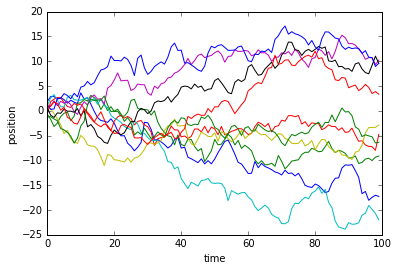
pandas
pandas, short for Python and data analysis (or panel datasets) was created by Wes McKinney, while he was working as a financial analyst (amongst other projects, he is currently working for Apache to get pandas to work with the Apache Arrow format). He initially began it as a port of R into Python for speed, but quickly diverged into a slightly different model.
It is primarily made for time series and tabular data, and its main point of use are the new classes, DataFrame and Series, modelled on Rs dataframe.
In [2]:
from pandas import Series, DataFrame
import pandas as pd
Series
Series are effectively NumPy arrays, but with an added index, which is retained through operations:
In [107]:
obj = Series([3,6,9,12])
obj
0 3
1 6
2 9
3 12
dtype: int64
In [256]:
#series are arrays, with an index:
obj.values
obj.index
#indexes are immutable!
obj.index[1] = 5
---------------------------------------------------------------------------
TypeError Traceback (most recent call last)
<ipython-input-256-1f81be84565f> in <module>()
3 obj.index
4 #indexes are immutable!
----> 5 obj.index[1] = 5
C:\Anaconda3\lib\site-packages\pandas\core\index.py in __setitem__(self, key, value)
1128
1129 def __setitem__(self, key, value):
-> 1130 raise TypeError("Index does not support mutable operations")
1131
1132 def __getitem__(self, key):
TypeError: Index does not support mutable operations
You can think of a Series, as a fixed length, ordered dict, and we can easily convert a dict to a Series:
In [111]:
sdata = {'Ohio': 35000, 'Texas': 71000, 'Oregon': 16000, 'Utah': 5000}
Series(sdata)
Ohio 35000
Oregon 16000
Texas 71000
Utah 5000
dtype: int64
In [259]:
#or:
l = Series([35000,71000,16000,5000], index=['Ohio','Texas','Oregon','Utah'])
print(l)
#indices must be unique~!
Ohio 35000
Texas 71000
Oregon 16000
Utah 5000
dtype: int64
In [118]:
#subsetting by index
l['Ohio']
35000
In [120]:
#can use all our numpy stuff! And retain our indexes
l[l.values > 30000]
Ohio 35000
Texas 71000
dtype: int64
In [260]:
#reindex with index, fills as NaN
k = Series(l, index=['Ohio','Texas','Oregon','Ontario'])
k
Ohio 35000
Texas 71000
Oregon 16000
Ontario NaN
dtype: float64
In [132]:
#NaN is the NA/missing for pandas!
k.isnull()
None == None
np.nan == np.nan
False
In [261]:
#add - watch, NaN overwrites!
k + l
Ohio 70000
Ontario NaN
Oregon 32000
Texas 142000
Utah NaN
dtype: float64
DataFrames
DataFrames are similar to a dict of a series - technically they are a 2d series with some linking between levels.
Columns are arrays (must be one data type), and rows are similar to dicts.
However, the row/column mapping is not as strictly enforced as R.
In [3]:
dat = pd.read_csv("http://jeremy.kiwi.nz/pythoncourse/assets/tests/r&d/test1data.csv")[1:20]
dat| TripType | VisitNumber | Weekday | Upc | ScanCount | DepartmentDescription | FinelineNumber | |
|---|---|---|---|---|---|---|---|
| 1 | 30 | 7 | Friday | 60538815980 | 1 | SHOES | 8931 |
| 2 | 30 | 7 | Friday | 7410811099 | 1 | PERSONAL CARE | 4504 |
| 3 | 26 | 8 | Friday | 2238403510 | 2 | PAINT AND ACCESSORIES | 3565 |
| 4 | 26 | 8 | Friday | 2006613744 | 2 | PAINT AND ACCESSORIES | 1017 |
| 5 | 26 | 8 | Friday | 2006618783 | 2 | PAINT AND ACCESSORIES | 1017 |
| 6 | 26 | 8 | Friday | 2006613743 | 1 | PAINT AND ACCESSORIES | 1017 |
| 7 | 26 | 8 | Friday | 7004802737 | 1 | PAINT AND ACCESSORIES | 2802 |
| 8 | 26 | 8 | Friday | 2238495318 | 1 | PAINT AND ACCESSORIES | 4501 |
| 9 | 26 | 8 | Friday | 2238400200 | -1 | PAINT AND ACCESSORIES | 3565 |
| 10 | 26 | 8 | Friday | 5200010239 | 1 | DSD GROCERY | 4606 |
| 11 | 26 | 8 | Friday | 88679300501 | 2 | PAINT AND ACCESSORIES | 3504 |
| 12 | 26 | 8 | Friday | 22006000000 | 1 | MEAT - FRESH & FROZEN | 6009 |
| 13 | 26 | 8 | Friday | 2236760452 | 1 | PAINT AND ACCESSORIES | 7 |
| 14 | 26 | 8 | Friday | 88679300501 | -1 | PAINT AND ACCESSORIES | 3504 |
| 15 | 26 | 8 | Friday | 2238400200 | 2 | PAINT AND ACCESSORIES | 3565 |
| 16 | 26 | 8 | Friday | 3019294203 | 1 | PAINT AND ACCESSORIES | 2801 |
| 17 | 26 | 8 | Friday | 72450408840 | 1 | PAINT AND ACCESSORIES | 1028 |
| 18 | 26 | 8 | Friday | 25541500000 | 2 | DAIRY | 1305 |
| 19 | 26 | 8 | Friday | 2310010776 | 1 | PETS AND SUPPLIES | 3300 |
In [4]:
# get the column names
dat.columns
#get the first five rows
dat.head()
#pick out specific columns
DataFrame(dat,columns=['TripType','VisitNumber'])
#same as
dat[['TripType','VisitNumber']]
#get one specific column
dat.TripType
#get one specific column
dat['TripType']
#use ix (index) to get the 10th row
dat.ix[10]
#add a new column
dat['foo']="spam"
#using other columns:
dat['foo'] = dat['VisitNumber'] + dat['ScanCount']
#add a new column with specific values
dat['foo']=Series(['spam', 'more spam'],index=[4,10])
In [159]:
#delete a column
del dat['foo']
#'http://pandas.pydata.org/pandas-docs/dev/generated/pandas.DataFrame.html'
In [43]:
#recall, indexes are immutable?
#how to reindex?
dat = dat.reindex(np.arange(5))
dat| TripType | VisitNumber | Weekday | Upc | ScanCount | DepartmentDescription | FinelineNumber | foo | |
|---|---|---|---|---|---|---|---|---|
| 0 | NaN | NaN | NaN | NaN | NaN | NaN | NaN | NaN |
| 1 | 30 | 7 | Friday | 60538815980 | 1 | SHOES | 8931 | 8 |
| 2 | 30 | 7 | Friday | 7410811099 | 1 | PERSONAL CARE | 4504 | 8 |
| 3 | 26 | 8 | Friday | 2238403510 | 2 | PAINT AND ACCESSORIES | 3565 | 10 |
| 4 | 26 | 8 | Friday | 2006613744 | 2 | PAINT AND ACCESSORIES | 1017 | 10 |
In [41]:
#can add defaults
dat.reindex(np.arange(7),fill_value=0)
dat.reindex(np.arange(10),method='ffill')| TripType | VisitNumber | Weekday | Upc | ScanCount | DepartmentDescription | FinelineNumber | foo | |
|---|---|---|---|---|---|---|---|---|
| 0 | NaN | NaN | NaN | NaN | NaN | NaN | NaN | NaN |
| 1 | 30 | 7 | Friday | 60538815980 | 1 | SHOES | 8931 | 8 |
| 2 | 30 | 7 | Friday | 7410811099 | 1 | PERSONAL CARE | 4504 | 8 |
| 3 | 26 | 8 | Friday | 2238403510 | 2 | PAINT AND ACCESSORIES | 3565 | 10 |
| 4 | 26 | 8 | Friday | 2006613744 | 2 | PAINT AND ACCESSORIES | 1017 | 10 |
| 5 | 26 | 8 | Friday | 2006613744 | 2 | PAINT AND ACCESSORIES | 1017 | 10 |
| 6 | 26 | 8 | Friday | 2006613744 | 2 | PAINT AND ACCESSORIES | 1017 | 10 |
| 7 | 26 | 8 | Friday | 2006613744 | 2 | PAINT AND ACCESSORIES | 1017 | 10 |
| 8 | 26 | 8 | Friday | 2006613744 | 2 | PAINT AND ACCESSORIES | 1017 | 10 |
| 9 | 26 | 8 | Friday | 2006613744 | 2 | PAINT AND ACCESSORIES | 1017 | 10 |
In [5]:
dat.drop(1)
dat.drop('foo', axis = 1)| TripType | VisitNumber | Weekday | Upc | ScanCount | DepartmentDescription | FinelineNumber | |
|---|---|---|---|---|---|---|---|
| 1 | 30 | 7 | Friday | 60538815980 | 1 | SHOES | 8931 |
| 2 | 30 | 7 | Friday | 7410811099 | 1 | PERSONAL CARE | 4504 |
| 3 | 26 | 8 | Friday | 2238403510 | 2 | PAINT AND ACCESSORIES | 3565 |
| 4 | 26 | 8 | Friday | 2006613744 | 2 | PAINT AND ACCESSORIES | 1017 |
| 5 | 26 | 8 | Friday | 2006618783 | 2 | PAINT AND ACCESSORIES | 1017 |
| 6 | 26 | 8 | Friday | 2006613743 | 1 | PAINT AND ACCESSORIES | 1017 |
| 7 | 26 | 8 | Friday | 7004802737 | 1 | PAINT AND ACCESSORIES | 2802 |
| 8 | 26 | 8 | Friday | 2238495318 | 1 | PAINT AND ACCESSORIES | 4501 |
| 9 | 26 | 8 | Friday | 2238400200 | -1 | PAINT AND ACCESSORIES | 3565 |
| 10 | 26 | 8 | Friday | 5200010239 | 1 | DSD GROCERY | 4606 |
| 11 | 26 | 8 | Friday | 88679300501 | 2 | PAINT AND ACCESSORIES | 3504 |
| 12 | 26 | 8 | Friday | 22006000000 | 1 | MEAT - FRESH & FROZEN | 6009 |
| 13 | 26 | 8 | Friday | 2236760452 | 1 | PAINT AND ACCESSORIES | 7 |
| 14 | 26 | 8 | Friday | 88679300501 | -1 | PAINT AND ACCESSORIES | 3504 |
| 15 | 26 | 8 | Friday | 2238400200 | 2 | PAINT AND ACCESSORIES | 3565 |
| 16 | 26 | 8 | Friday | 3019294203 | 1 | PAINT AND ACCESSORIES | 2801 |
| 17 | 26 | 8 | Friday | 72450408840 | 1 | PAINT AND ACCESSORIES | 1028 |
| 18 | 26 | 8 | Friday | 25541500000 | 2 | DAIRY | 1305 |
| 19 | 26 | 8 | Friday | 2310010776 | 1 | PETS AND SUPPLIES | 3300 |
In [180]:
#getting data
dat[['TripType','Upc']]
dat['ScanCount']>1
dat[dat['ScanCount']>1]| TripType | VisitNumber | Weekday | Upc | ScanCount | DepartmentDescription | FinelineNumber | foo | |
|---|---|---|---|---|---|---|---|---|
| 3 | 26 | 8 | Friday | 2238403510 | 2 | PAINT AND ACCESSORIES | 3565 | NaN |
| 4 | 26 | 8 | Friday | 2006613744 | 2 | PAINT AND ACCESSORIES | 1017 | spam |
| 5 | 26 | 8 | Friday | 2006618783 | 2 | PAINT AND ACCESSORIES | 1017 | NaN |
| 11 | 26 | 8 | Friday | 88679300501 | 2 | PAINT AND ACCESSORIES | 3504 | NaN |
| 15 | 26 | 8 | Friday | 2238400200 | 2 | PAINT AND ACCESSORIES | 3565 | NaN |
| 18 | 26 | 8 | Friday | 25541500000 | 2 | DAIRY | 1305 | NaN |
In [3]:
# as promised, .add with fill
l = Series([35000,71000,16000,5000], index=['Ohio','Texas','Oregon','Utah'])
k = Series(l, index=['Ohio','Texas','Oregon','Ontario'])
l = DataFrame(l, columns = ["pop"])
k = DataFrame(k, columns = ["pop"])
print(l+k)
print(l)
print(k)
l.add(k, fill_value=0)
pop
Ohio 70000
Ontario NaN
Oregon 32000
Texas 142000
Utah NaN
pop
Ohio 35000
Texas 71000
Oregon 16000
Utah 5000
pop
Ohio 35000
Texas 71000
Oregon 16000
Ontario NaN
| pop | |
|---|---|
| Ohio | 70000 |
| Ontario | NaN |
| Oregon | 32000 |
| Texas | 142000 |
| Utah | 5000 |
Summary
That’s it for today.
Next lesson we will cover in more detail how to read in and clean data, as well as merging, and the split, apply, combine methods on DataFrames.
Exercises
1. Create an array of size 10, with all 0s
2. Reshape the above vector to have dims of (5,2)
3. Create a 4*4 identity matrix in NumPy (use google or the docs for a function)
4. Create a 10 by 10 matrix or random values (randn, mean = 3), and find the minimum and maximum values. Find the index of these values
5. Normalise the above matrix to have a mean of 0
6. Create a Series, which has an index of NY, SF, TO, and CH, and the values 0.2, 0.9, 3.5 and 2.4
7. Reindex this series to include VA with NA
8. Add the two above Series, correcting for NaN