Installation Instructions

Introduction

Welcome to Python @ Precima!

Over the next 10 weeks, we will go over how to use Python for data science. We will cover data types and structures, syntax, the current data science stack, data visualisation, best practices for reproducibility of analysis, and so on.

We will be using Anaconda from continuum analytics as our Python distribution for this course. This is so we can start with a working Python platform, with iPython, Jupyter notebooks and an IDE, Spyder.

We will use Python 3.5 for the course, rather than 2.7 - Python 2.7 is due to hit end of life in 2020 and all of the data science stack is available in 3.5

Installation

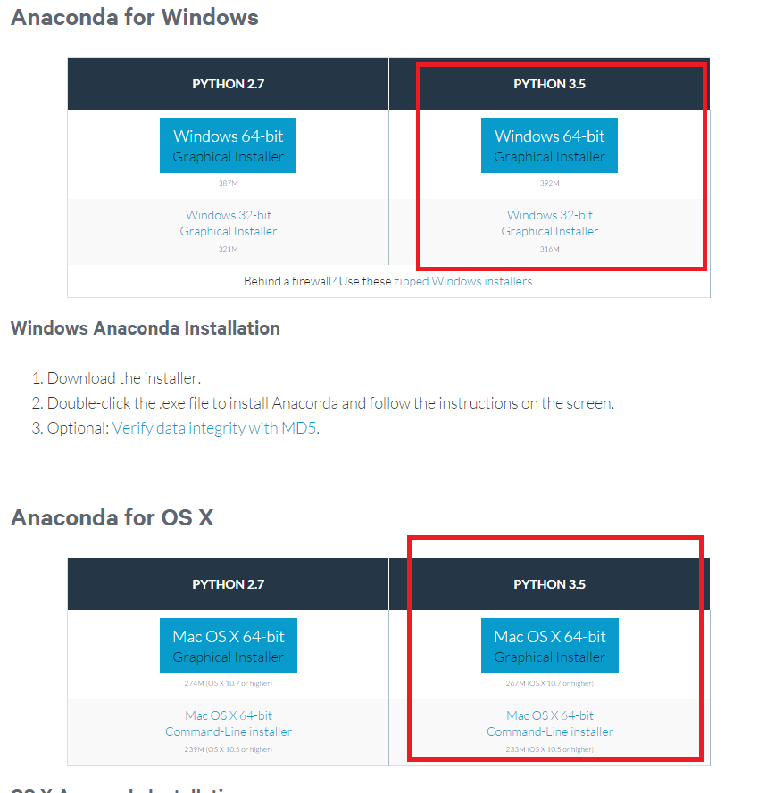
Go to the download page for anaconda and download the installer for your OS. Make sure you get the 3.5 version, not 2.7. Follow the installation instructions for your OS.

Verifying and Updating

From there, open your command line (use Windows Powershell or type ‘cmd’ in Start>Run) and enter:

conda --version

To check your install has worked. You should receive an output similar to:

conda 3.18.8

Indicating the install was successful. If not, please redownload and reinstall.

Now update conda:

conda update conda

Which will indicate if there are updates available and prompt you to update.

Once updated, check the version of Python you have:

python --version

Hopefully giving you something like this:

Python 3.5.1 :: Anaconda 2.4.1 (64 bit)

If not, make sure you downloaded the correct version above, or make sure you know why (if you are using another version of Python).

Using conda, we can also install alternate environments, for a walk-through of how to use Python 2.7 as well as 3.5 see this website

Included Programs

Anaconda provides us with 3 useful Python programs, ipython-notebook, ipython- qtconsole and spyder-app (We will not use glueviz or orange).

Open the Anaconda launcher. If you are on windows it will be in the start menu, on OSX and linux, you can type launcher at the command prompt. If this does not work, try installing the launcher and retrying:

conda install -f launcher
conda install -f node-webkit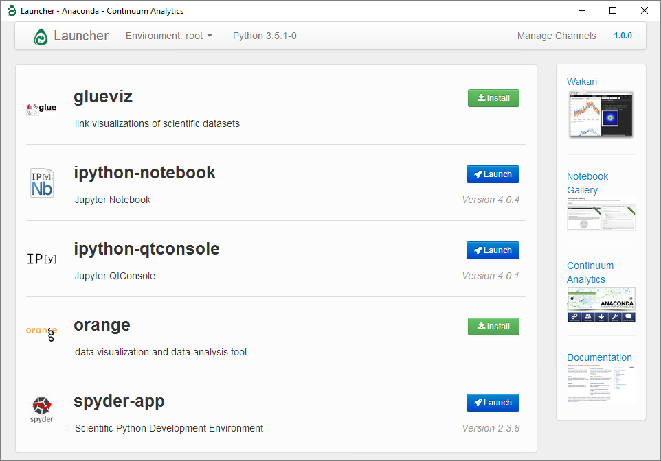

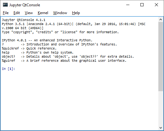
iPython-QtConsole

iPython-QtConsole an advanced interpreter, with the large number of included modules of iPython and the ability to include graphics. Launch it:

In the window, type out the following commands (don’t worry if you don’t understand them yet). You should get the following graph in your window.

import matplotlib.pyplot as plt
%matplotlib inline
plt.plot([1, 2, 3, 23, 32, 2, 1]);
plt.ylabel('Y');
plt.xlabel('X');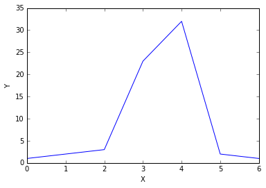

Spyder

Spyder is an IDE for Python, and allows us to write, run and troubleshoot scripts interactively. Launch Spyder:

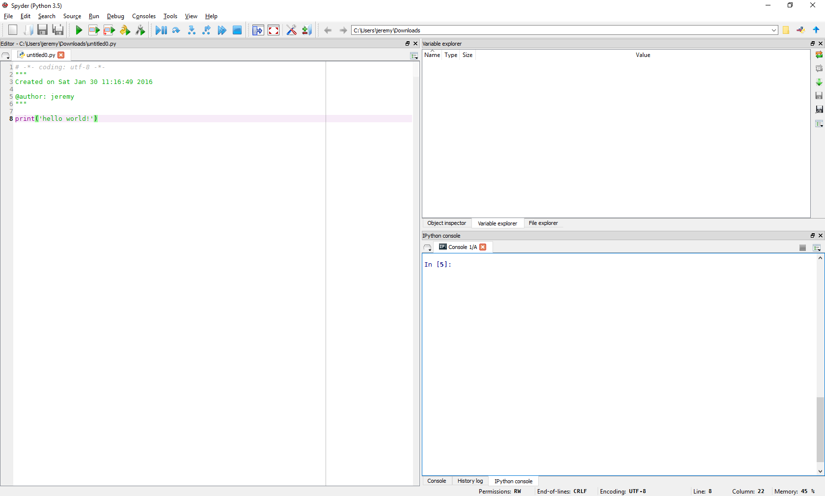
The large left pane is a script editor, the right upper pane allows us to explore the variables, objects and functions we have in memory, and the right lower pane is an iPython console, similar to the iPython-QtConsole. In the script window, enter in: print(“Hello World!”) below the comments, save the script and click run.

iPython Notebooks

iPython Notebooks (currently undergoing a rebranding into Jupyter Notebooks) are JSON formatted documents, which contain cells of content. These cells can be markdown, HTML, code or a number of other formats. These documents are then run locally as a webpage, linked to kernel to allow coding inside the browser. In our case, the code is Python, through a connection to an iPython kernel, but development now allows a wide range of languages (R, Haskell, Julia, etc. ) instead of or in addition to Python. We will discuss iPython notebooks in much greater detail later in the course.

These instructions are written in a notebook, download them here - download, unzip, then open ipython-notebook. It should launch a browser window pointing to http://localhost:8888/tree if not, click the link to open it:

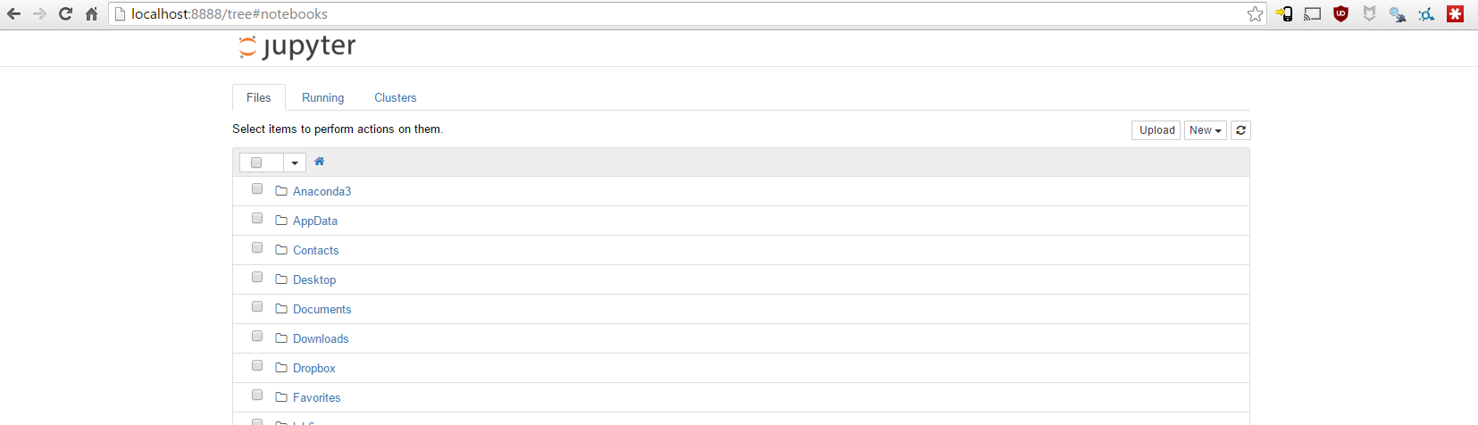
This is a locally served webpage, no files leave your local computer.

Browse to where you downloaded the above file, and open it by clicking on it.

It will look very similar to this document, but you know have a toolbar at the top, and you can edit the code/text (you will need to double click the text to get the raw markdown). You can execute a cell of code using ctrl-enter

Once you have played around a little, try evaluating the below code a couple of times, and see if you can guess what is being simulated.

import matplotlib.pyplot as plt
import numpy as np
%matplotlib inline

steps, repeats = 100, 10
t = np.arange(steps)
stepstaken = 0.01 * np.random.randn(steps, repeats)
positions = stepstaken.cumsum(axis = 0)
plt.plot(positions);
plt.xlabel('time');
plt.ylabel('position');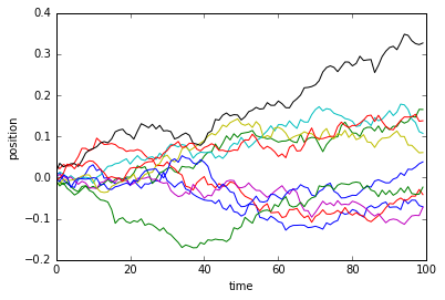

Wrap-up

You should now have installed Python 3.5, and taken a brief tour of the 3 interfaces we will use for the rest of the course.

If anything gave errors, the first step is to uninstall, redownload the installer and reinstall. If you are still having problems, ask one of your colleagues, or leave a comment in the comment box below (NB please be aware, comments are hosted on disqus and public, please do not give out any senstive information).